Adventures in Hybrid Rendering
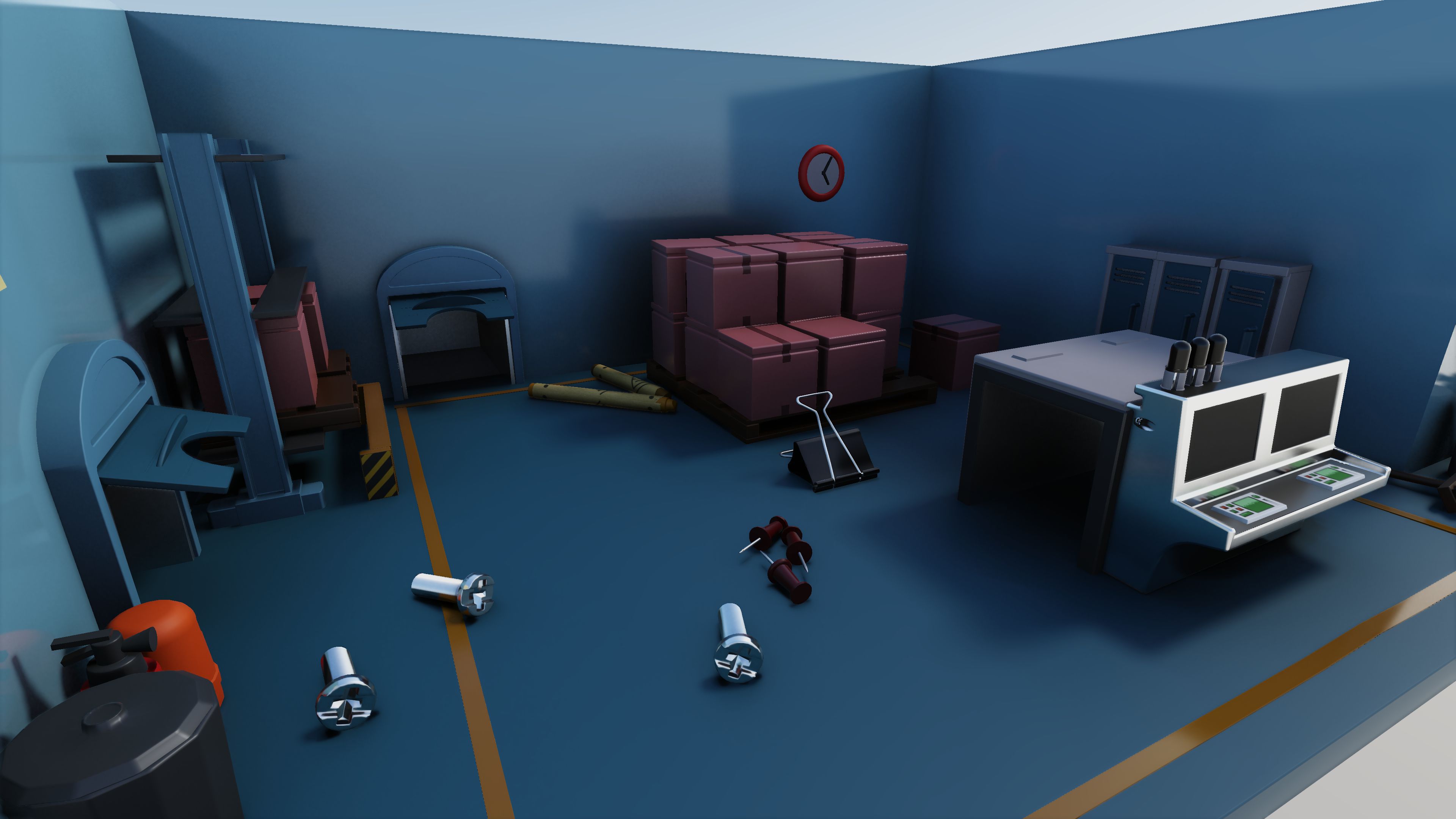
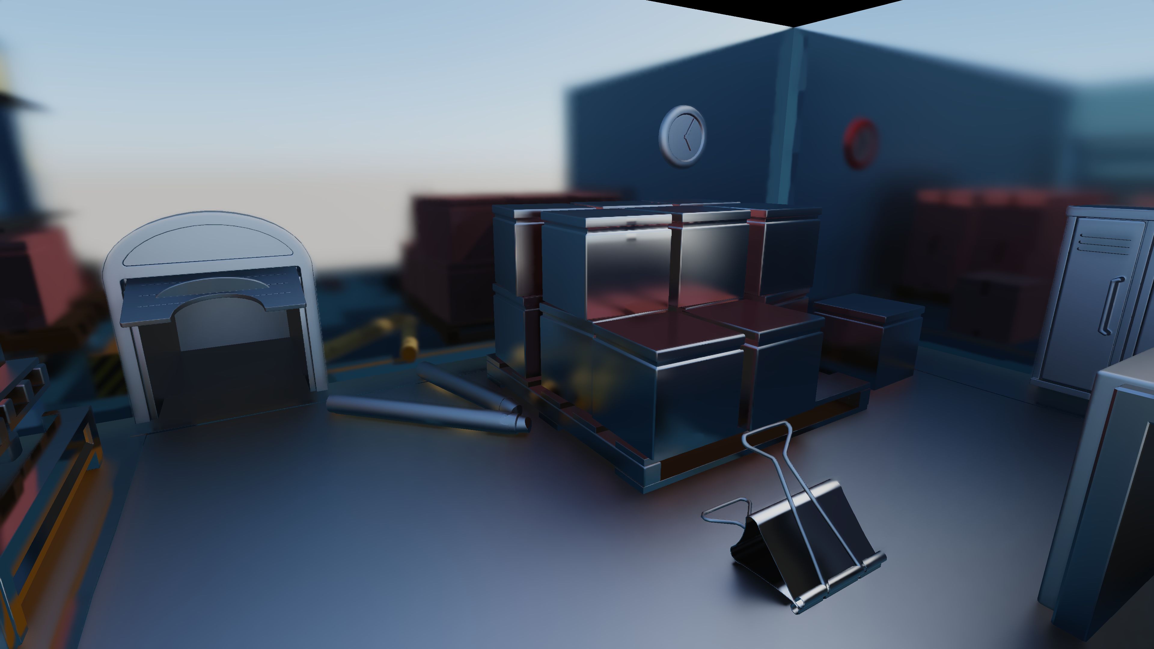
As an accompanying piece to my recently released Hybrid Rendering sample, this blog post dives into some of the techniques and optimizations used and will help anyone interested to understand the project.
Before going any further let’s answer the question “Why hybrid rendering?”. In a typical rasterization based rendering pipeline, certain effects such as Global Illumination, Reflections and Soft Shadows have to be approximated using either screen space techniques, offline baking or other approaches which typically lead to less-than-believable results in many cases. A fully ray traced renderer on the other hand would be able to model these real-life phenomena much more realistically, although at a heavy performance hit.
Hybrid Rendering is simply the best of both worlds; meaning that we’re enhancing a Rasterization based pipeline by bolting on a bunch of Ray Traced effects that would otherwise have to be done using approximations or hacks.
Denoising
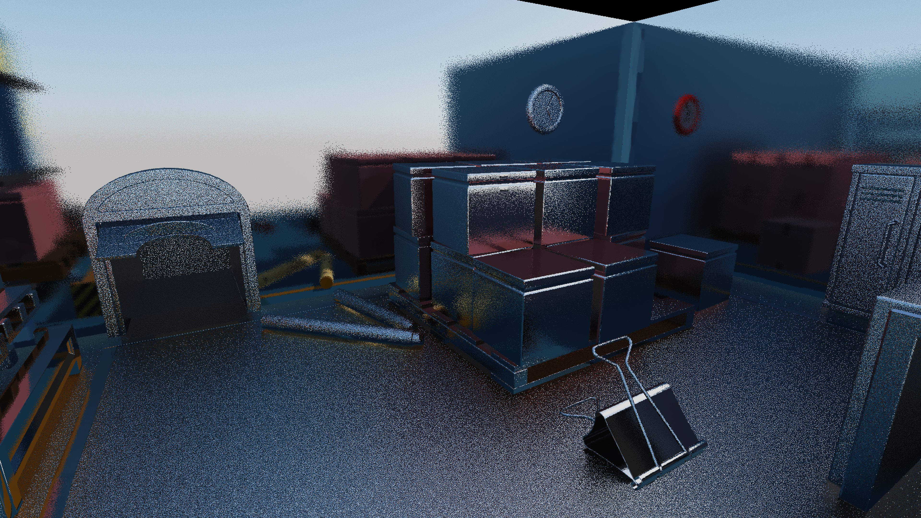
Since real-time rendering applications have a tight frame time budget, adding ray tracing to the mix means that our ray budget for a single frame needs to be kept to a minimum in order to hit our frame rate target. Because of this, the rays-per-pixel number, or more commonly known as samples-per-pixel (spp), is usually 1 or 2 for most techniques.
While such a low ray count is great performance-wise, visually it results in a noisy output especially for effects with some randomness such as Soft Shadows or Glossy Reflections. They simply cannot be rendered correctly with just a single ray per-frame. This is where denoising comes in, which attempts to take the noisy output of the ray tracing pass and clean it up using filters.
The main denoising algorithm used in this sample is based on Spatiotemporal Variance-Guided Filtering (SVGF) [1]. The algorithm is split into two main parts: Temporal and Spatial filtering. The sections below will try to explain SVGF in a simplified way for dummies such as myself. If you’re looking for the gory details, please do read the original paper.
Temporal Filtering
Even though we can only afford to shoot one ray per pixel in our use case, we can get around this limitation by accumulating samples over time, meaning that we can reuse older samples to create a cleaner, less noisy image. This is done by essentially finding where the current pixel was in the previous frame and then accumulating the current pixel into that history sample.
The way we find where the pixel was in the previous frame is by using the current pixels motion vector which will allow us to find where this particular pixel was during the previous frame in screen space.
The following simplified code block runs through the basic temporal accumulation logic.
// Fetch the current sample.
vec4 current_sample = texture(s_Current, tex_coord);

// Get the motion vector for the current pixel.
vec2 motion_vector = texture(s_MotionVector, tex_coord).rg;

// Compute the history coordinate.
vec2 history_coord = tex_coord + motion_vector;

// Initialize the output to the current sample in case reprojection fails.
vec4 output = current_sample;

// Initialize history length, which is the number of frames that the sample has been accumulated over.
float history_length = 1.0f;

// Check if the history sample is valid.
if (is_reprojection_valid(history_coord))
{
    // Fetch history sample
    vec4 history_sample = texture(s_History, history_coord);

    // Fetch the length of the history sample and increment by 1 since the sample will be accumulated
    history_length = texture(s_HistoryLength, history_coord).r + 1.0f;

    // Compute the alpha value which will be used to determine how much of the history sample will be used
    float alpha = 1.0f / history_length;

    // Accumulate the sample
    output = mix(history_sample, current_sample, alpha);
}

imageStore(i_Output, coord, output);
imageStore(i_OutputHistoryLength, coord, vec4(history_length, 0.0f, 0.0f, 0.0f));
The is_reprojection_valid() function basically checks if the history sample can actually be reprojected or not. One such reason for a failed reprojection is due the the history sample being off screen, which mainly happens when moving or rotating the camera.
But another trickier reason for this is due to disocclusion, which is when the sample was occluded in the past but is now visible in the current frame, therefore no valid history exists.
In order to check the validity of the history sample, it is necessary to have certain pixel properties from the previous frame available to us. To that end, my sample ping-pongs between two G-Buffers: one containing this frames' data, one containing the history data required for reprojection.
Now let’s take a look at the various disocclusion checks used in this sample.
Plane Distance
While it might make sense to use depth to determine if the surface belonging to the current pixel is too far away in the previous frame, this can result in false negatives if the camera is viewing a surface at a grazing angle.
A better way to determine this was proposed by NVIDIA in their Recurrent Blur presentation [2] where you check if the current and history sample both reside on the same plane.
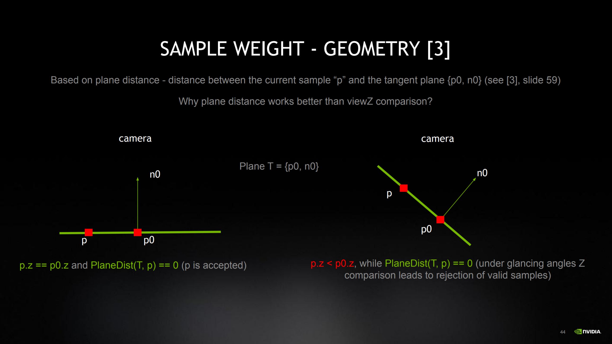
Diagram showing the difference between comparing depth values vs Plane Distance values from NVIDIA
This solves the false negative reprojections we get when using depth based comparisons. A dot product is used to determine the distance between the two planes and if it is within the threshold value it is considered to be valid.
bool plane_distance_disocclusion_check(vec3 current_pos, vec3 history_pos, vec3 current_normal)
{
    vec3  to_current    = current_pos - history_pos;
    float dist_to_plane = abs(dot(to_current, current_normal));

    return dist_to_plane > PLANE_DISTANCE_THRESHOLD;
}
Normal
Another way to determine if the history sample is valid is to check if the angle between both world space normals is below a certain threshold. This would mean that the history sample belongs to the same surface as the current sample.
bool normals_disocclusion_check(vec3 current_normal, vec3 history_normal)
{
    if (pow(abs(dot(current_normal, history_normal)), 2) > NORMAL_DISTANCE_THRESHOLD)
        return false;
    else
        return true;
}
Mesh ID
While the two previous disocclusion checks are sufficient by themselves, there is also another check which compares the mesh ID of the current and history sample. This mesh ID is simply a unique integer assigned to each submesh in the scene and written into the G-Buffer. This check will guarantee that both samples originate from the same surface, especially in the case of moving objects. However, make sure to keep the mesh ID’s consistent between frames as otherwise this comparison does not make sense.
bool mesh_id_disocclusion_check(float mesh_id, float mesh_id_prev)
{
    if (mesh_id == mesh_id_prev)
        return false;
    else
        return true;
}
Pixel Variance
As the SVGF name suggests, variance plays a rather important role in this denoiser. And here we are talking about the variance of each pixel over time. During the temporal accumulation pass this variance is stored as the first and second moments of the current sample’s luminance (or in the case of shadows or ambient occlusion, the value itself). These moments are also accumulated over time like the color itself, which allows the subsequent blur pass to dynamically adjust depending on how noisy the output is.
// compute first two moments of luminance
vec2 moments = vec2(0.0f);
moments.r    = luminance(color);
moments.g    = moments.r * moments.r;

// temporal integration of the moments
moments = mix(history_moments, moments, alpha_moments);
After the moments are accumulated, the actual variance value that will be read by the Spatial filter is computed and written out.
float variance = max(0.0f, moments.g - moments.r * moments.r);
Spatial Filtering
The spatial filtering portion of SVGF uses the À-Trous wavelet filter which is essentially a blur with multiple iterations where you accumulate pixels further from the center with each subsequent iteration.
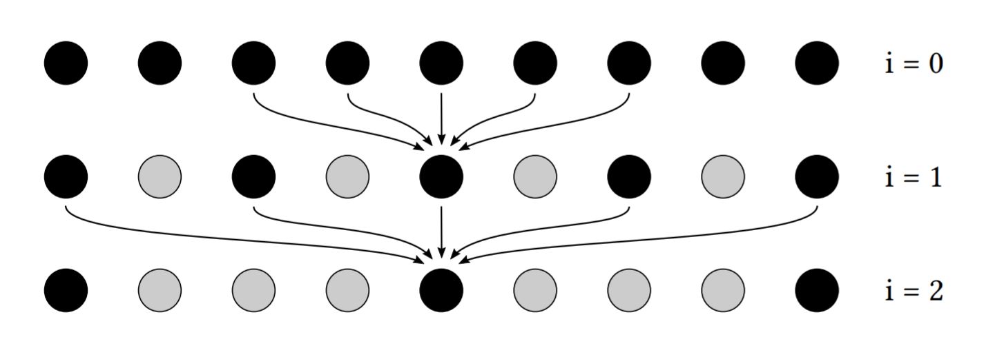
Illustration of the first three iterations of a 1D À-Trous Wavelet Transform, courtesy of NVIDIA
If that doesn’t help you visualize the filter behavior, here’s the same thing in code-form.
for (int yy = -FILTER_RADIUS; yy <= FILTER_RADIUS; yy++)
{
    for (int xx = -FILTER_RADIUS; xx <= FILTER_RADIUS; xx++)
    {
        // STEP SIZE = 1 << filter_iteration
        const ivec2 sample_coord = coord + ivec2(xx, yy) * STEP_SIZE;

        // Apply filter...
    }
}
In order to prevent over-blurring and to preserve edge details, each sample is weighted using the variance as well as some edge-stopping weights similar to the disocclusion checks in the temporal pass.
float normal_edge_stopping_weight(vec3 center_normal, vec3 sample_normal, float power)
{
    return pow(clamp(dot(center_normal, sample_normal), 0.0f, 1.0f), power);
}

float depth_edge_stopping_weight(float center_depth, float sample_depth, float phi)
{
    return exp(-abs(center_depth - sample_depth) / phi);
}

float luma_edge_stopping_weight(float center_luma, float sample_luma, float phi)
{
    return abs(center_luma - sample_luma) / phi;
}
The phi value for the luma_edge_stopping_weight() function is derived from the variance that we calculated at the end of the temporal pass.
// u_PushConstants.phi_color is set to 10.0f by default
float phi_color = u_PushConstants.phi_color * sqrt(max(0.0, EPSILON + variance));
For this sample, around 3-4 À-Trous filter iterations seem to be sufficient for decent results with good performance.
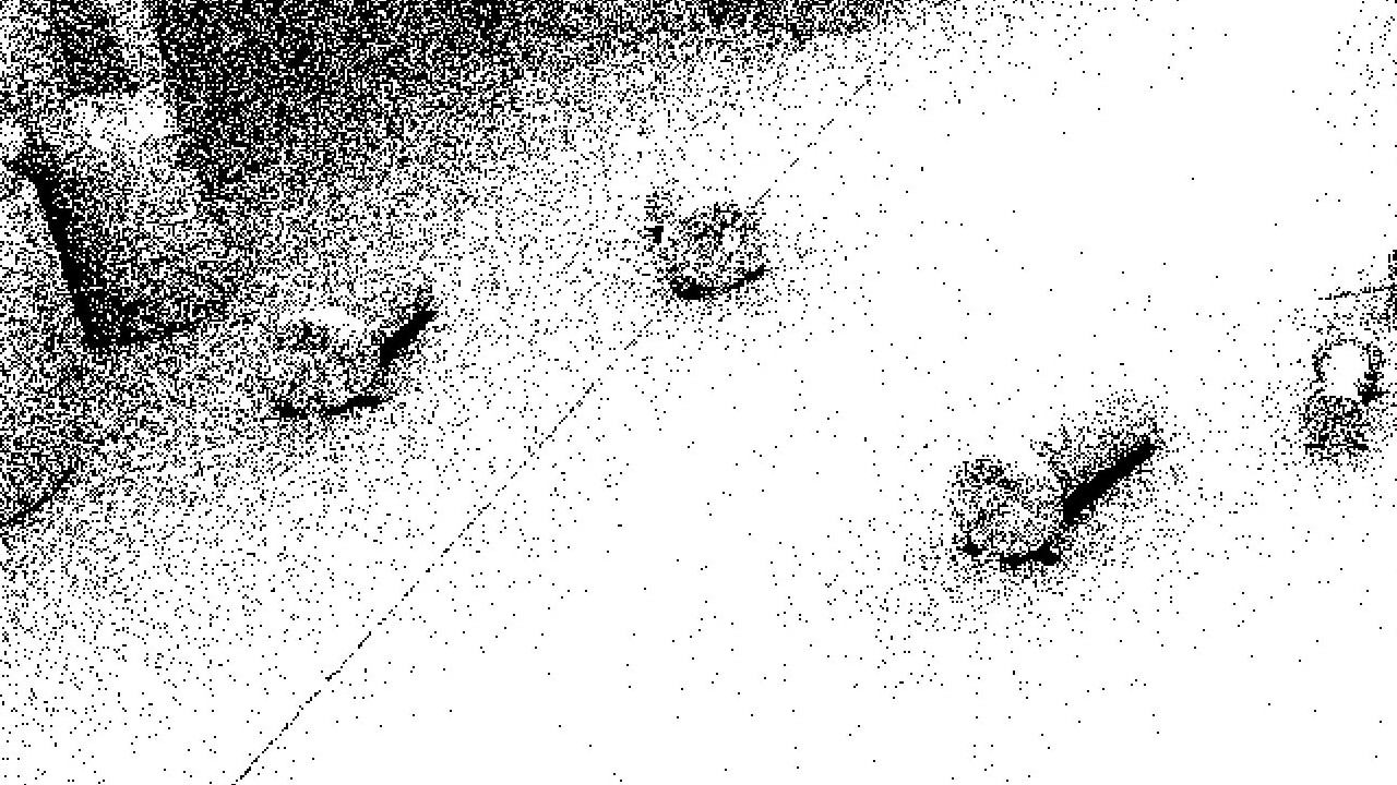
Tile-Based Denoising
While it is simpler to just use the denoiser across the entire frame, it does put a strain on performance as it requires a lot of texture fetches. To reduce the performance impact of this, we can choose to only denoise the pixels that actually need denoising. In this sample we make this decision at the tile level. This means that the screen is split up into tiles and for each tile we will consider all the ray traced input values and decide whether there is at least a single pixel within this tile that requires denoising. If so, we will write out the tile coordinates into a buffer and atomically incrementing the number of tiles that require denoising. After this we can perform a compute dispatch for only the tiles that require denoising by using an indirect dispatch combined with the buffer containing the tile coordinates.
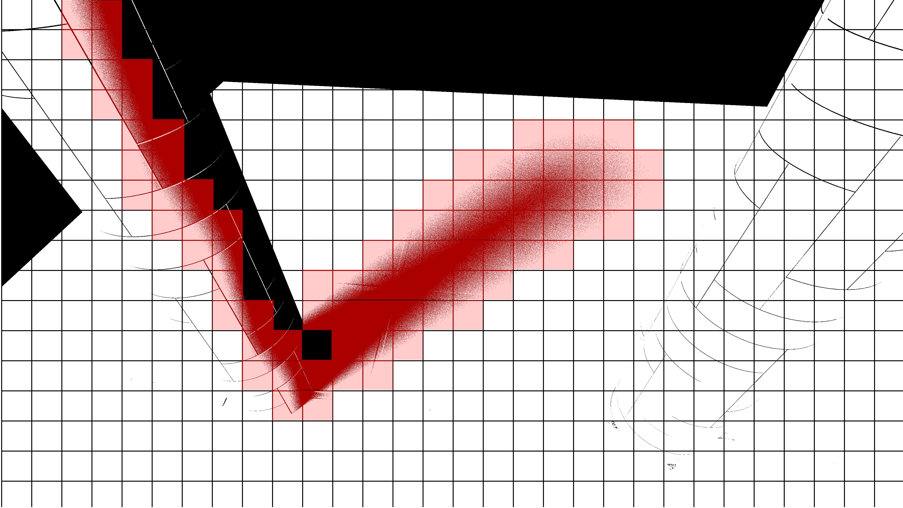
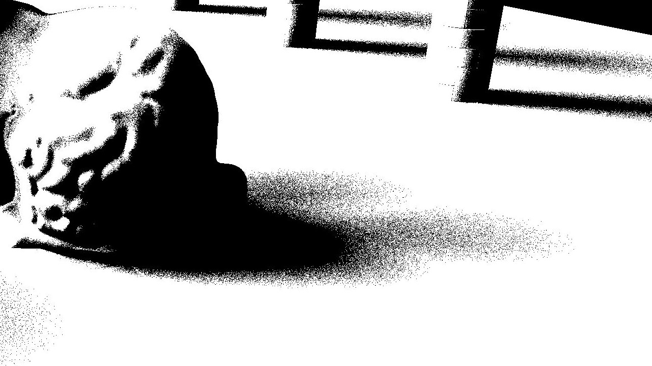
Simplified visualization of classifying penumbra tiles for denoising Ray Traced Soft Shadows.
How a tile is considered for denoising depends entirely on the technique, so the following sections for each technique will cover their respective denoising details.
Sampling
The initial sampling strategy for the ray generation stages was white noise which, while producing adequate results, results in some slight animated noise after both Temporal and Spatial filtering. Significantly better results can be obtained by using the Blue Noise sampler introduced in the paper “A Low-Discrepancy Sampler that Distributes Monte Carlo Errors as a Blue Noise in Screen Space” [3]. The output using this Blue Noise sampler is more spatially coherent which makes the output a lot cleaner after some blurring compared to using White Noise.

The sampler implementation can be found in the files blue_noise.h, blue_noise.cpp and bnd_sampler.glsl and was taken from the author’s Unity sample.
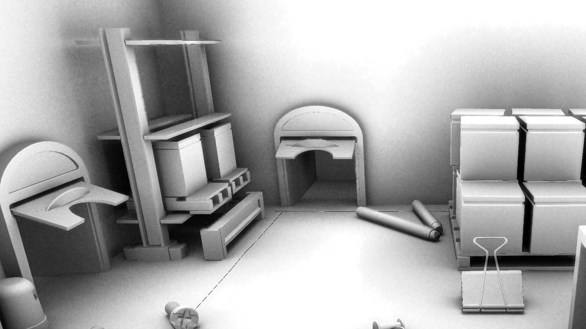
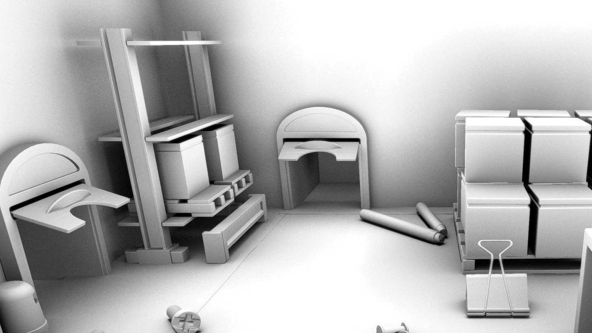
Soft Shadows
Ray Traced Soft Shadows
Now let’s look at some actual implementation details for the Ray Traced effects in the sample, starting with Soft Shadows. The main problem with regular PCF filtered shadow maps is the fact that you don’t get the nice soft penumbra you would usually get with something like a large area light. Of course you can approximate it using Percentage Closer Soft Shadows but the blocker search in that technique is only a poor approximation of the actual penumbra you’d get in something like a path tracer, while having all the usual shadow mapping artefact to go with it. Ray Traced Soft Shadows on the other hand gives perfect penumbras free of peter panning or shadow acne artefact.
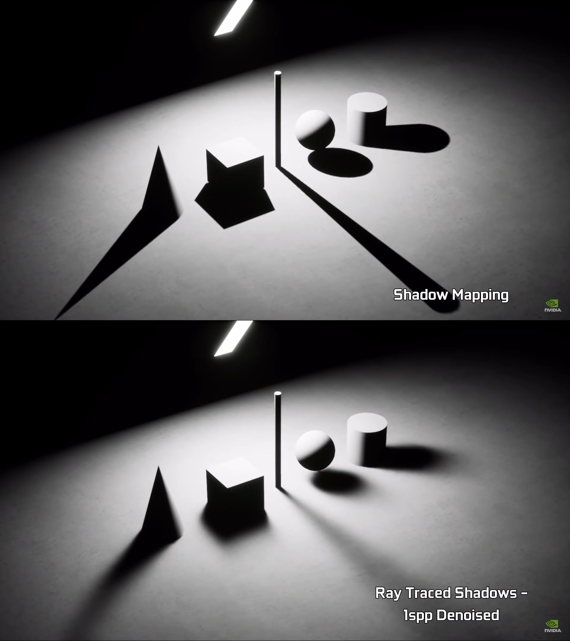
Comparison of Shadow Maps and Ray Traced Soft Shadows from NVIDIA
To simplify the actual implementation, the actual ray tracing is done in a compute shader using ray queries instead of the full ray tracing pipeline, since shadows does not require much complex ray tracing capabilities. The lack of setting up the Shader Binding Table makes the code relatively more readable as well.
Ray Generation
Since physically based soft shadows require an area light, which means that there is more than a single direction than we can fire a ray towards, an infinite number of directions actually. But since we’re limited to a single ray per pixel, we have to randomly pick a direction towards the light aka randomly sample the light source. There’s many ways to achieve this, but for this demo I used the method from the blue noise master Alan Wolfe’s blog post [4].
// Fetch a blue noise value for this frame.
vec2 rnd_sample      = next_sample(current_coord);

vec3 light_dir       = light_direction(light);

vec3 light_tangent   = normalize(cross(light_dir, vec3(0.0f, 1.0f, 0.0f)));
vec3 light_bitangent = normalize(cross(light_tangent, light_dir));

// calculate disk point
float point_radius = light_radius(light) * sqrt(rng.x);
float point_angle  = rng.y * 2.0f * M_PI;
vec2  disk_point   = vec2(point_radius * cos(point_angle), point_radius * sin(point_angle);

Wi = normalize(light_dir + disk_point.x * light_tangent + disk_point.y * light_bitangent);
Optimisations
I’ve also borrowed an interesting trick from the AMD FidelityFX Shadow Denoiser [5] where they pack 32 ray hit results from an 8x4 portion of the screen into a 32-bit uint output image. This works out perfectly for shadows since the result of the visibility ray query is either true or false. Since I’m using compute shaders for ray tracing, the local size is set to (8, 4, 1) so that each work group perfectly fits 32 rays. So each thread can trace a ray and bitwise-or the result into a shared variable that the first thread can write out into the output image once every thread has finished execution.
shared uint g_visibility;

uint result = 0;

// Trace ray and store result...

atomicOr(g_visibility, result << gl_LocalInvocationIndex);

barrier();

if (gl_LocalInvocationIndex == 0)
    imageStore(i_Output, ivec2(gl_WorkGroupID.xy), uvec4(g_visibility));
The beauty of packing the rays like this is that during the temporal accumulation pass, it makes it easier for us to do a really wide neighborhood clamp with very little texture fetches. And in this case, it’s a 17x17 neighborhood. The FidelityFX Denoiser also calculates the neighborhood mean with a separable approach. For each thread we compute the horizontal mean across 17 pixels centered around the current pixel, meaning 8 pixels to the left and right. We also compute the horizontal mean values 8 pixels above and below the current x-value. We then store these values in shared memory, exposing them to the other threads in the work group. Once all the threads are past this point we can vertically gather the horizontal means from the earlier step to get the final neighborhood mean value. As you can probably tell by now, this greatly reduces the number of texture fetches you’d usually need.
// Compute horizontal mean values.
float top    = horizontal_neighborhood_mean(ivec2(coord.x, coord.y - 8));
float middle = horizontal_neighborhood_mean(ivec2(coord.x, coord.y));
float bottom = horizontal_neighborhood_mean(ivec2(coord.x, coord.y + 8));

// Store horizontal mean values in shared memory.
g_mean_accumulation[gl_LocalInvocationID.x][gl_LocalInvocationID.y]      = top;
g_mean_accumulation[gl_LocalInvocationID.x][gl_LocalInvocationID.y + 8]  = middle;
g_mean_accumulation[gl_LocalInvocationID.x][gl_LocalInvocationID.y + 16] = bottom;

barrier();

float mean = 0.0f;

// Gather horizontal mean values.
for (int y = 0; y <= 16; y++)
    mean += g_mean_accumulation[gl_LocalInvocationID.x][gl_LocalInvocationID.y + y];

// Divide by weight to get the final neighborhood mean value.
return mean / weight;
The denoiser is also optimized to only run on tiles that contain at least a single penumbra shadow value, meaning that the variance that we calculate in SVGF is greater than 0.0 for any thread. A shared memory value is used as a flag which gets set by any of the threads in the work group if the condition is met. If denoising is needed, the tile coordinate is written to a buffer. If no denoising is needed, we write the tile coordinate to another buffer which contains a list of tiles that are fully in shadow. Afterwards we clear the final shadow mask image to white, then run an indirect compute dispatch to output 0.0 for the fully shadowed tiles, then finally denoise only the tiles that need it by running another indirect compute dispatch using the buffer we wrote to before.
// If all the threads are in shadow, skip the À-Trous filter.
if (depth != 1.0f && output_visibility_variance.x > 0.0f)
    g_should_denoise = 1;

barrier();

if (gl_LocalInvocationIndex == 0)
{
    if (g_should_denoise == 1)
    {
        uint idx                   = atomicAdd(DenoiseTileDispatchArgs.num_groups_x, 1);
        DenoiseTileData.coord[idx] = current_coord;
    }
    else
    {
        uint idx                  = atomicAdd(ShadowTileDispatchArgs.num_groups_x, 1);
        ShadowTileData.coord[idx] = current_coord;
    }
}
Performance
- NVIDIA GeForce RTX 2070 SUPER
- 1920x1080 Window Resolution
- Full Resolution Ray Trace
- Sponza Scene
| Pass | Original | Optimized |
|---|---|---|
| Ray Trace | 0.52 ms | 0.3 ms |
| Temporal Accumulation | 0.37 ms | 0.36 ms |
| A-Trous Filter | 1.48 ms | 0.55 ms |
| Total | 2.39 ms | 1.23 ms |
Ambient Occlusion
Ray Traced Ambient Occlusion
The Ambient Occlusion implementation in this sample is essentially the same as soft shadows, except with a slightly simplified denoiser. It still uses the 32 ray packing trick from AMD and also the same 17x17 neighborhood clamp with separable mean calculation. Where the denoiser differs is in the Spatial Filtering aspect which is only using a simple separable gaussian blur. I felt that the added complexity and performance hit of the full on À-Trous filter is not necessary for Ambient Occlusion and my assumption held up for the most part. However you do see some slight animated noise when looking at the AO by itself, probably due to the lack of variance driven blurring.
The cost of AO is further cut down thanks to running it at a quarter size, or half resolution, of the back buffer. Since Ambient Occlusion is very diffuse-looking by nature, the upscaling doesn’t have any negative effects on it, other than scaling up the noise artifacts, but it’s nothing a good blur can’t soften up. In addition to this I’m using a simple Bilateral Upsample using depth and normals to preserve edges in the output image without bleeding the occlusion values all over the place.

As for the actual ray tracing pass itself, it’s really nothing special here. 1spp as usual, with rays generated in a uniformly sampled cosine lobe. The secret sauce really is in the use of blue noise which greatly improves the effectiveness of the denoiser. The remaining noise in the output image can probably be gotten rid of with the use of a second temporal pass such as a temporal pre-pass or a TAA-style stabilization pass such as the one from NVIDIA’s Recurrent Blur Denoiser.
Optimisations
The tile-based optimization used here is similar to the one from Soft Shadows, but it only needs one indirect dispatch since AO doesn’t usually have massive fully shadowed areas as you’d see with shadows, so if a tile has at least a single AO value below 1.0, we mark that tile for denoising and write the tile coords. The rest is the same as before.
// If at least one thread has an occlusion value, perform denoising.
if (out_ao < 1.0f)
    g_should_denoise = 1;

barrier();

if (g_should_denoise == 1 && gl_LocalInvocationIndex == 0)
{
    uint idx                   = atomicAdd(DenoiseTileDispatchArgs.num_groups_x, 1);
    DenoiseTileData.coord[idx] = current_coord;
}
Performance
- NVIDIA GeForce RTX 2070 SUPER
- 1920x1080 Window Resolution
- Quarter Resolution Ray Trace
- Sponza Scene
| Pass | Original | Optimized |
|---|---|---|
| Ray Trace | 0.093 ms | 0.09 ms |
| Temporal Accumulation | 0.09 ms | 0.091 ms |
| Blur | 0.12 ms | 0.06 ms |
| Total | 0.53 ms | 0.46 ms |
Reflections
Ray Traced Reflections
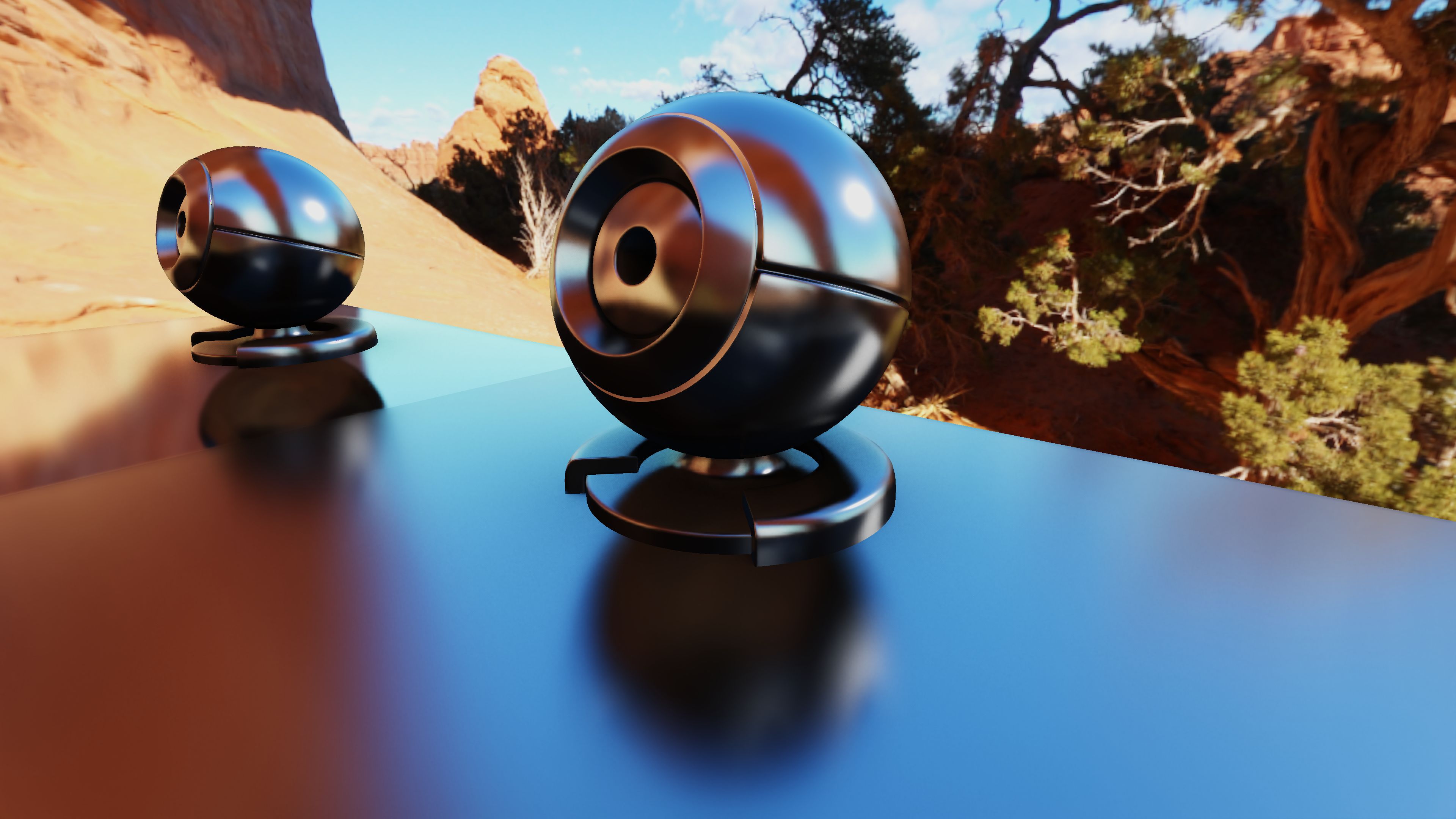
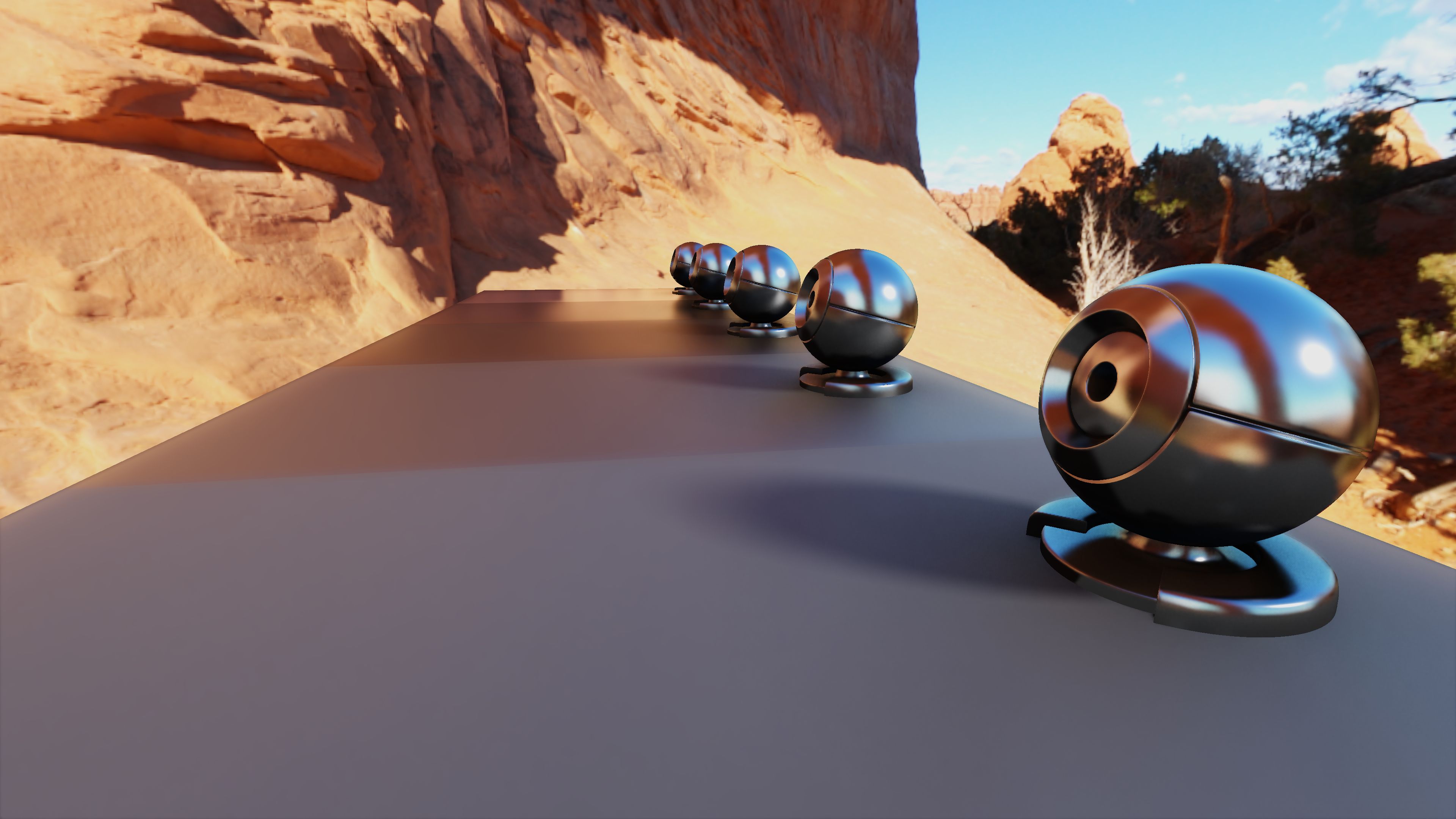
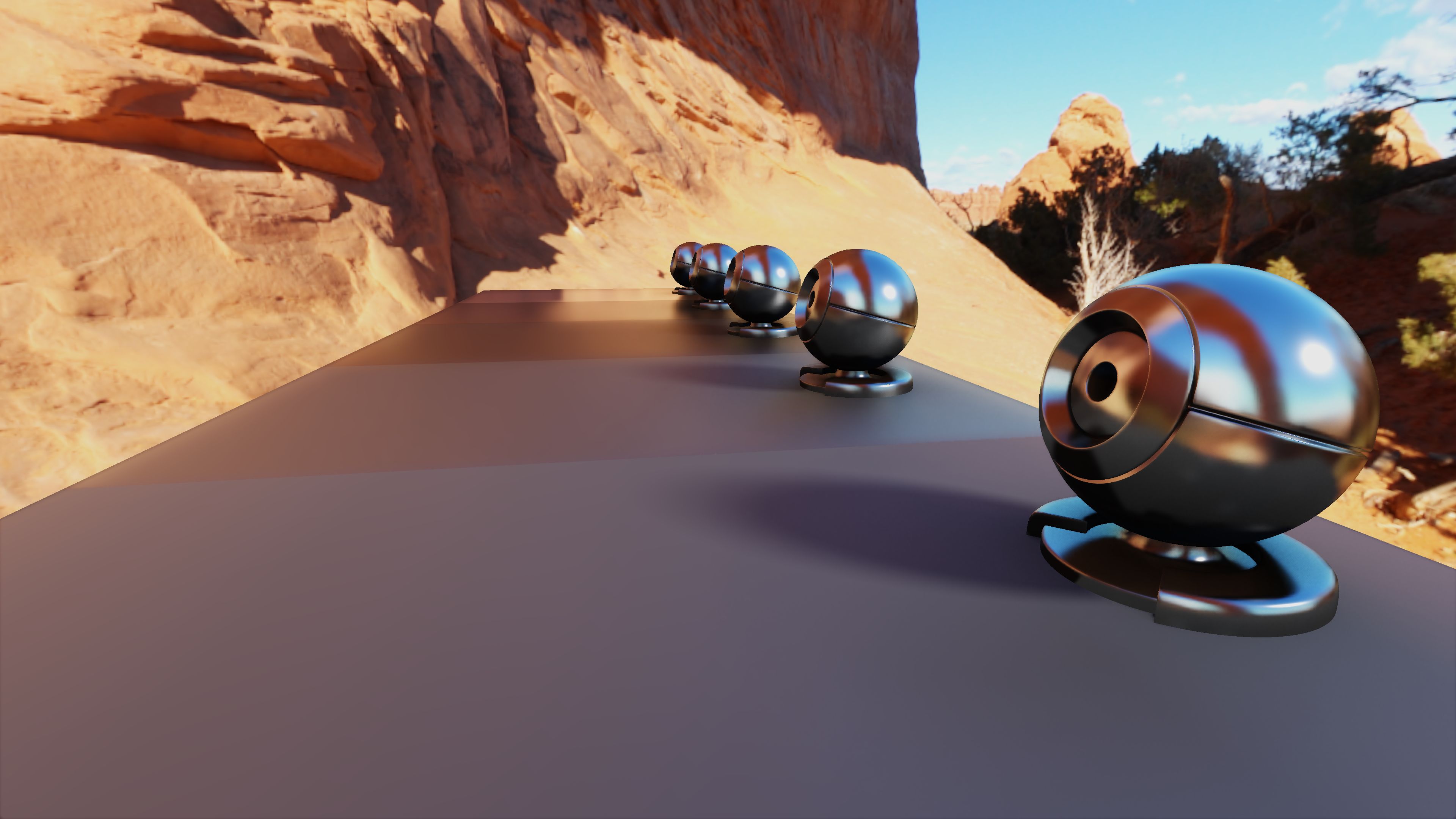
Now this is where things start getting interesting. The implementation here is quite straightforward, with the ray tracing done with an RT pipeline as opposed to a ray query because it will let me handle more complex cases such as alpha testing more easily. The rays are generated by importance sampling the GGX microfacet BRDF and uses a single bounce. Denoising is done through SVGF with a slight twist to the temporal reprojection pass which I will go into a bit further on.
Reprojection
Typical temporal reprojection is done by taking the current pixels' motion vector and subtracting it from the screen space position. Let’s call this “Surface Point Reprojection”. While this works fine for reprojecting diffuse techniques such as shadows, AO and GI, anything that is view-dependent such as reflections will have some issues on certain objects when reprojected using this technique. This is because of the whole parallax effect you’d see when inspecting reflections while moving your viewpoint around. Using Surface Point Reprojection we would end up with a ton of ghosting and smearing when moving the camera around.
Let’s think, what do we really need for reprojecting reflections? We need to know where the surface that is reflected within the current pixel was located in the previous frame, not where the current pixel itself was located in the previous frame. This is quite the tough problem to solve and many people have taken a crack at it, such as [6] and most recently [7] from Ray Tracing Gems by the fine folks over at UL Benchmarks.
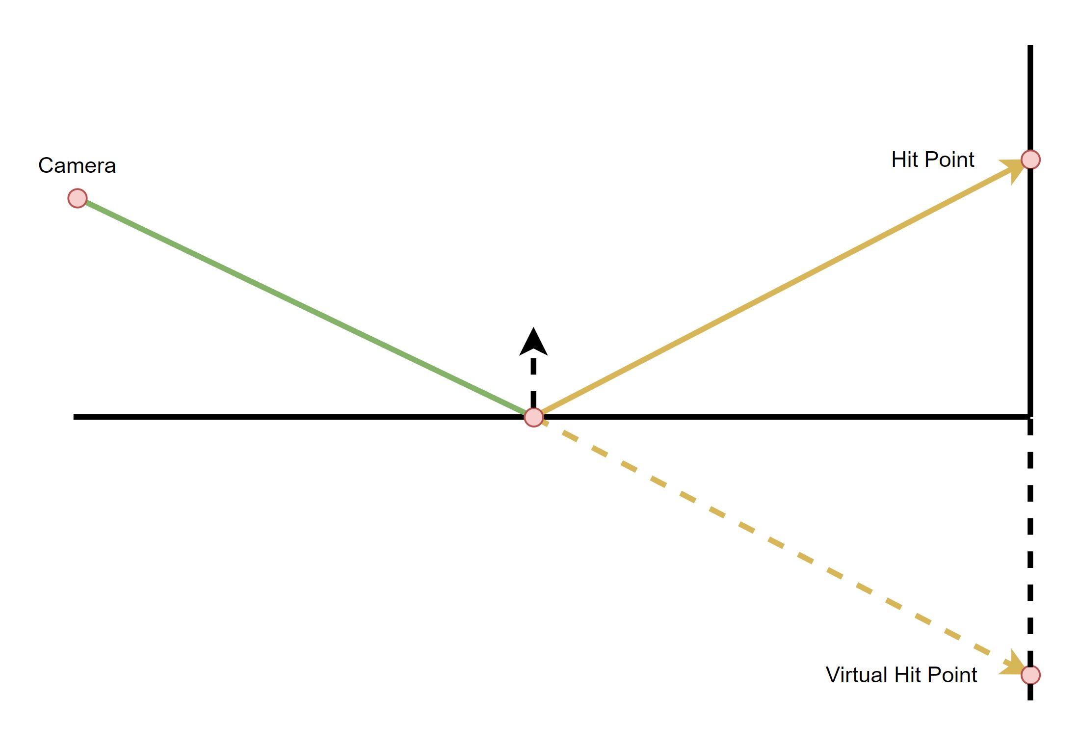
Illustration of the Virtual Hit Point used to reproject Ray Traced Reflections
While those ideas seem great, they are also quite complicated and I just couldn’t wrap my head around it. So I went ahead and borrowed another idea from the FidelityFX Denoiser. How they achieve Hit Point Reprojection is by storing the ray hit distance in the ray tracing pass, and in the reprojection pass using that distance to extending the primary ray into the surface, which essentially gives us the Virtual Position of the reflected point. Now if we take this Virtual Position and transform it reproject it into screen space using the previous frames' View Projection matrix it would roughly give us where the Virtual Position was in the previous frame in screen space coordinates, which is exactly what we are looking for.
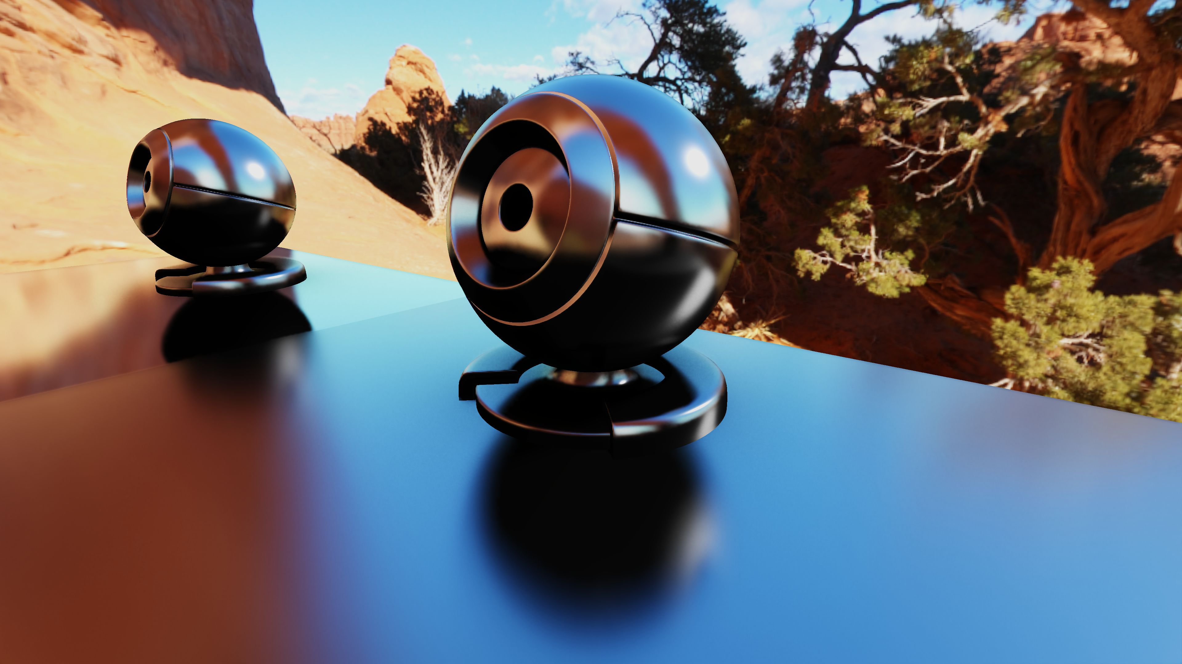
As you can see it does quite a decent job at reprojecting reflections on flat surfaces, but does tend to breakdown on curved surfaces. A solution for this was mentioned in the Hybrid Rendering for Real-Time Ray Tracing chapter by SEED in Ray Tracing Gems [8] where they described using two different reprojection techniques: Hit Point Reprojection on flat surfaces and Surface Reprojection on curved surfaces. This solution proved quite effective on my sample as well.
But how did I determine the curvature of a surface you say? Well, let me present to you what I like to call ‘The Poor Man’s Curvature Estimation’ which is just an approximation using the partial derivatives of the geometric normal and written out into the G-Buffer.
float compute_curvature(float interpolated_normal)
{
    vec3 dx = dFdx(interpolated_normal);
    vec3 dy = dFdy(interpolated_normal);

    float x = dot(dx, dx);
    float y = dot(dy, dy);

    return pow(max(x, y), 0.5f);
}
Indirect Lighting
When shading the hit points in the ray tracing pass it’s not enough to just do direct lighting because that by itself will make the reflections in shadows regions look pitch black. Of course, you can get away with a fixed ambient term but we can get better and more accurate looking results by using proper indirect diffuse and specular. For diffuse I’m using the DDGI probes generated in the current frame which really helps lighten up the darker areas.
For specular we could use another ray bounce but since this is a real-time renderer we really have to try and keep the ray count down to a minimum, so because of that I’m just sampling the prefiltered environment map similar to how we would sample indirect specular with Image Based Lighting. This can definitely lead to light leaking, especially in indoor scenes which is why it is a good idea to instead sample local reflection probes instead of a global reflection probe so that the indirect specular would more closely match the lighting of the surrounding environment. But for the purposes of this demo a single global prefiltered environment map fits the bill.
Optimisations
Because the denoising process is quite expensive I try not to denoise pixels that don’t actually require any denoising. For example, if a pixel has zero roughness, the generated rays will be equal to a perfect specular reflection, or in other words a perfect mirror. Since mirror reflections are already perfectly converged at 1spp, we can just skip the denoiser for such pixels. To reduce the need for the denoiser even more, I’ve added a mirror reflection threshold value that basically makes pixels with roughness values within a certain delta value of 0.0 behave as mirror reflections. By default this value is set to 0.05, so any surface with values below 0.05 will receive mirror reflections and will not need any denoising. Not only does this reduce time from the denoiser, it also makes the rays more coherent in these regions, meaning that they will all travel in the same direction, resulting in ray hits that are closer together. This means that threads in a warp will have a greater chance of sampling the same texture and geometry, allowing for better cache utilization.
if (roughness < MIRROR_REFLECTIONS_ROUGHNESS_THRESHOLD)
{
    vec3 R = reflect(-Wo, N.xyz);

    // Trace a ray along mirror reflection direction.
    traceRayEXT(u_TopLevelAS, ray_flags, cull_mask, 0, 0, 0, ray_origin, tmin, R, tmax, 0);
}
else
{
    vec2 Xi = next_sample(current_coord) * u_PushConstants.trim;

    vec4 Wh_pdf = importance_sample_ggx(Xi, N, roughness);

    float pdf = Wh_pdf.w;
    vec3  Wi  = reflect(-Wo, Wh_pdf.xyz);

    // Trace a ray along an importance sampled direction.
    traceRayEXT(u_TopLevelAS, ray_flags, cull_mask, 0, 0, 0, ray_origin, tmin, Wi, tmax, 0);
}
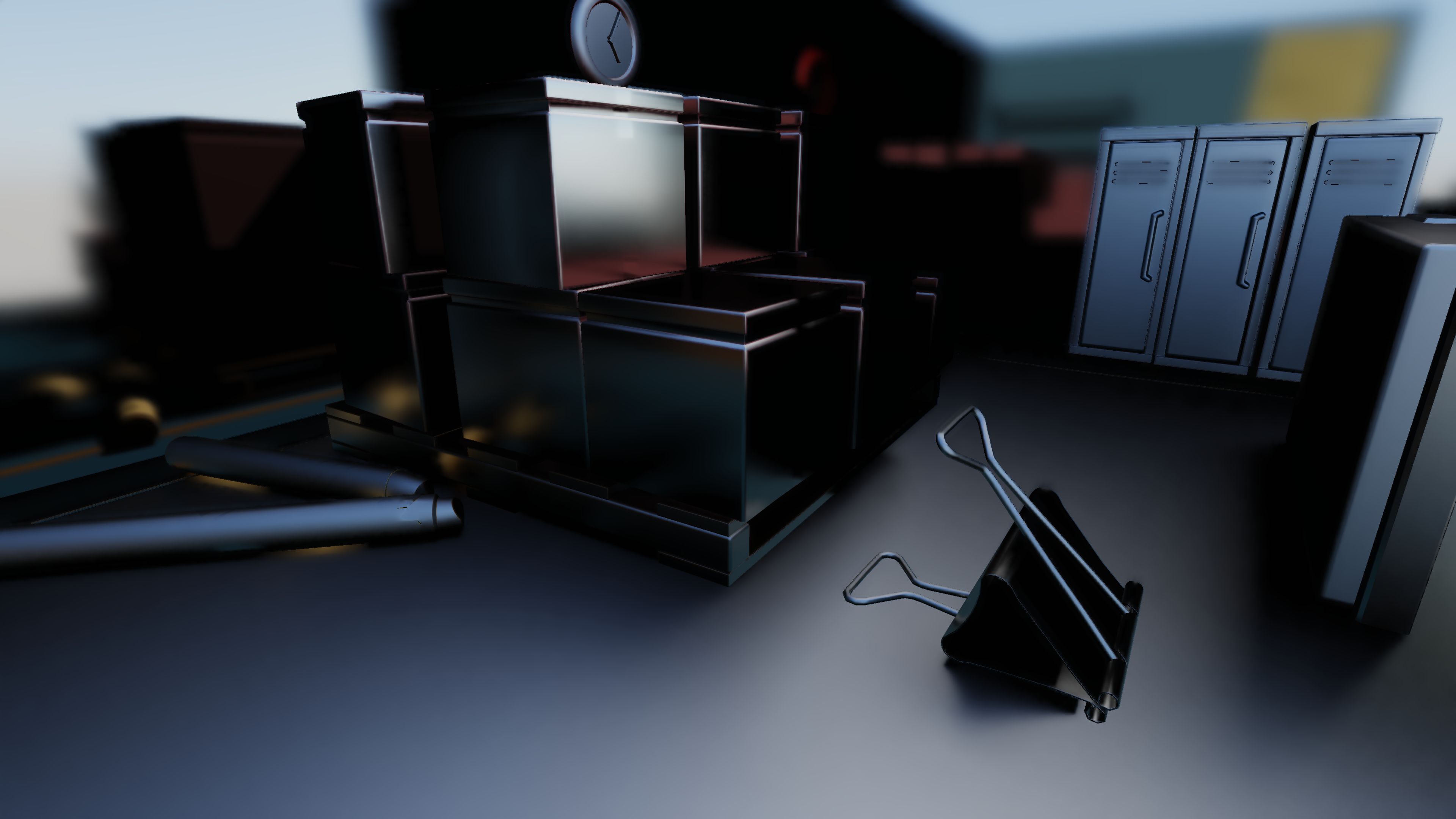
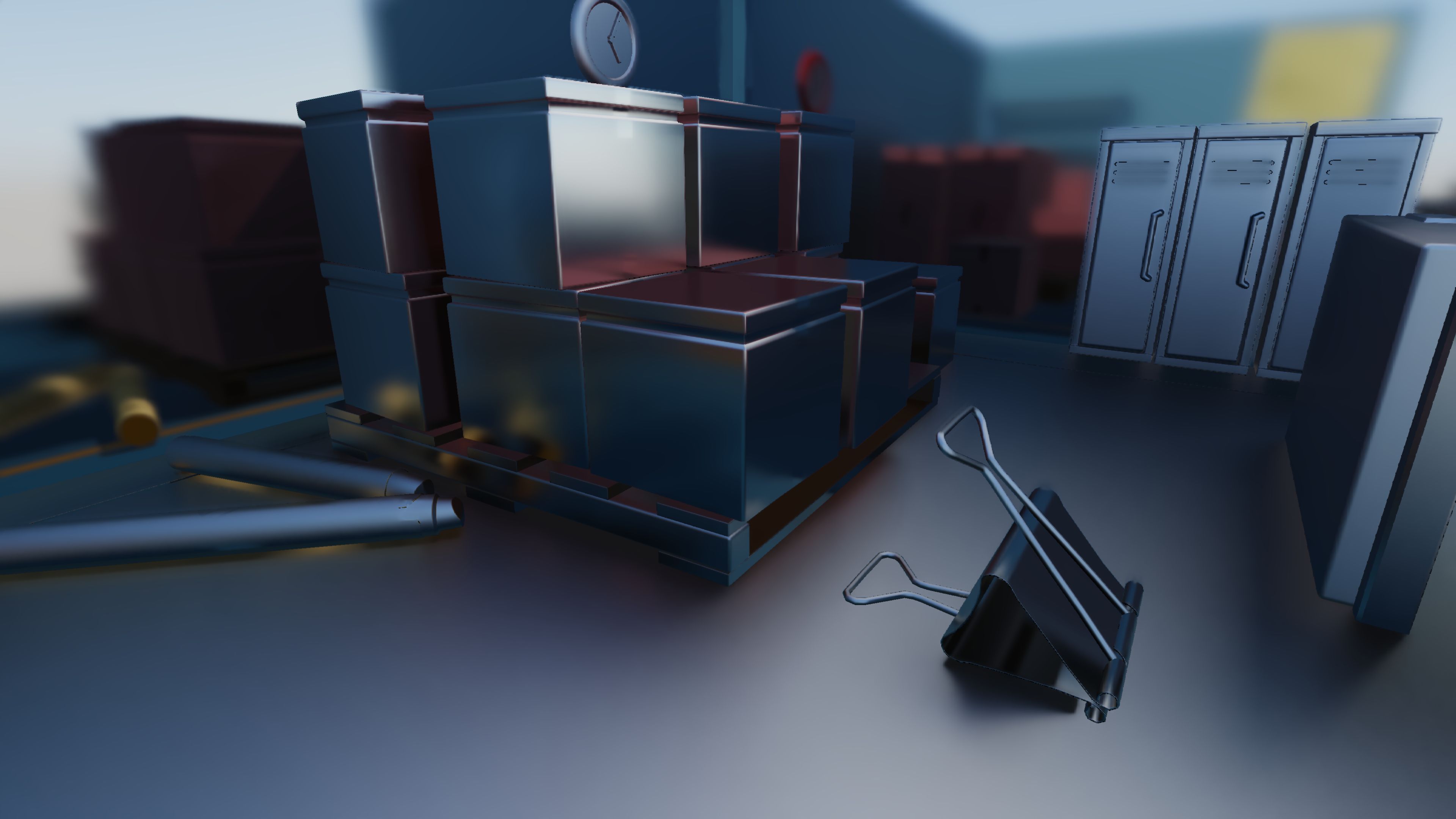
Similarly, when the roughness value is past a certain point the reflection becomes rather diffuse as the ray directions are quite spread out. I’ve used this to approximate the reflections of pixels with a roughness value above a certain threshold using the DDGI probes. While not being a perfect match to the fully ray traced result, it’s a decent enough approximation as can be seen below. The beauty of this is that you don’t even need to trace the ray for these pixels. You can simply check the roughness value, and if it is above this threshold you can sample the DDGI probes and directly write the output into the image. And there is no need to denoise these pixels either. However you do loose out on shadows within reflections in those regions, but it isn’t a big deal since fully rough surfaces are pretty much diffuse so you can rely on the shadow mask for any shadows.
As always the denoising here is done on a per-tile basis; tiles that need denoising are put into one buffer and the tiles that only require a straight up copy into another. Both are then executed with an indirect compute dispatch. Copy shader just directly copies the output from the temporal accumulation pass into the final output image. A tile is said to need denoising if there is at least a single pixel between the Mirror Reflection Threshold and the DDGI Approximation Threshold.
// If all the threads are in within the roughness range, skip the À-Trous filter.
if (depth != 1.0f && roughness >= MIRROR_REFLECTIONS_ROUGHNESS_THRESHOLD)
{
    if (u_PushConstants.approximate_with_ddgi == 1)
    {
        if (roughness <= DDGI_REFLECTIONS_ROUGHNESS_THRESHOLD)
            g_should_denoise = 1;
    }
    else
        g_should_denoise = 1;
}

barrier();

if (gl_LocalInvocationIndex == 0)
{
    if (g_should_denoise == 1)
    {
        uint idx                   = atomicAdd(DenoiseTileDispatchArgs.num_groups_x, 1);
        DenoiseTileData.coord[idx] = current_coord;
    }
    else
    {
        uint idx                = atomicAdd(CopyTileDispatchArgs.num_groups_x, 1);
        CopyTileData.coord[idx] = current_coord;
    }
}
Performance
- NVIDIA GeForce RTX 2070 SUPER
- 1920x1080 Window Resolution
- Half Resolution Ray Trace
- Sponza Scene
| Pass | Original | Optimized |
|---|---|---|
| Ray Trace | 1.41 ms | 1.08 ms |
| Temporal Accumulation | 0.6 ms | 0.57 ms |
| A-Trous Filter | 0.38 ms | 0.25 ms |
| Total | 2.61 ms | 2.13 ms |
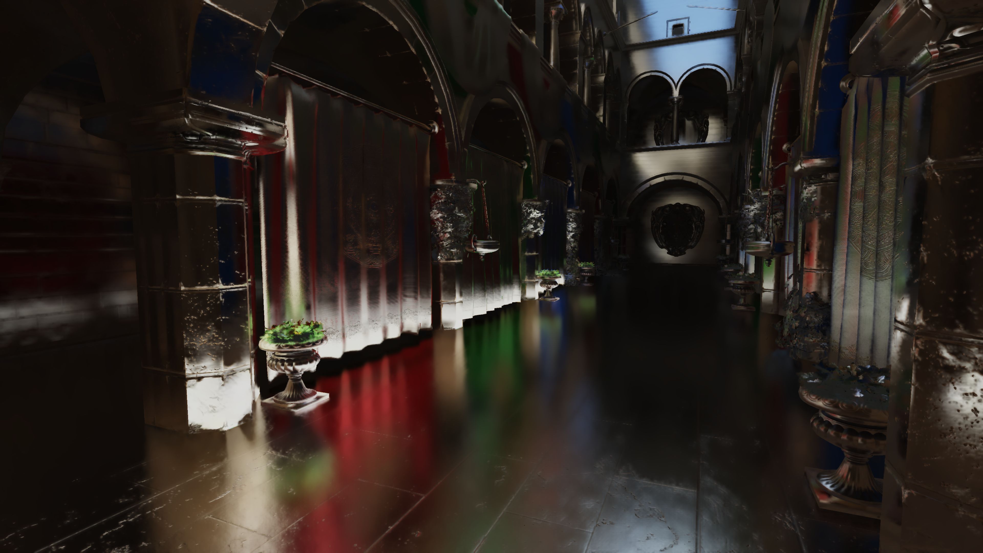
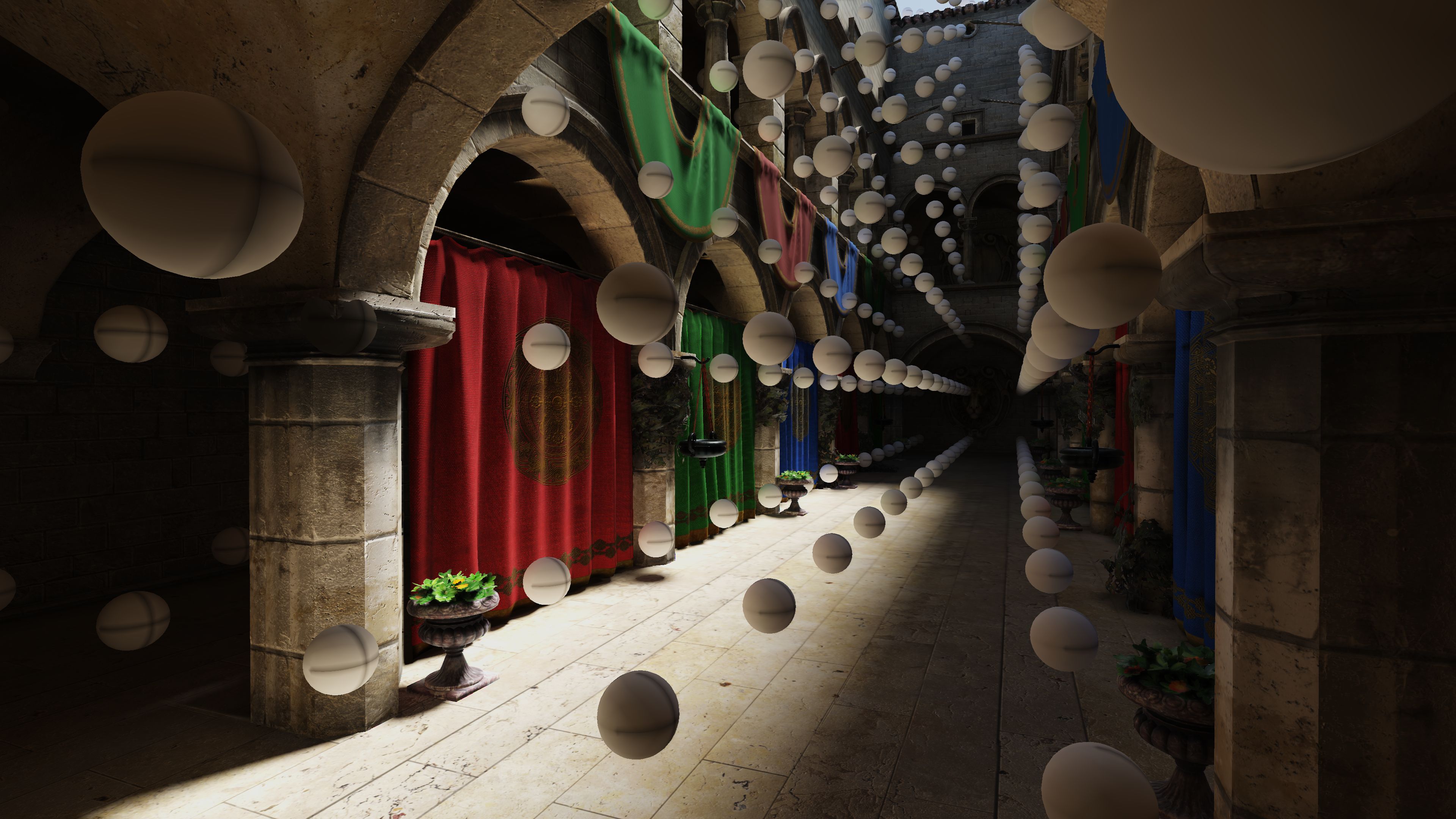
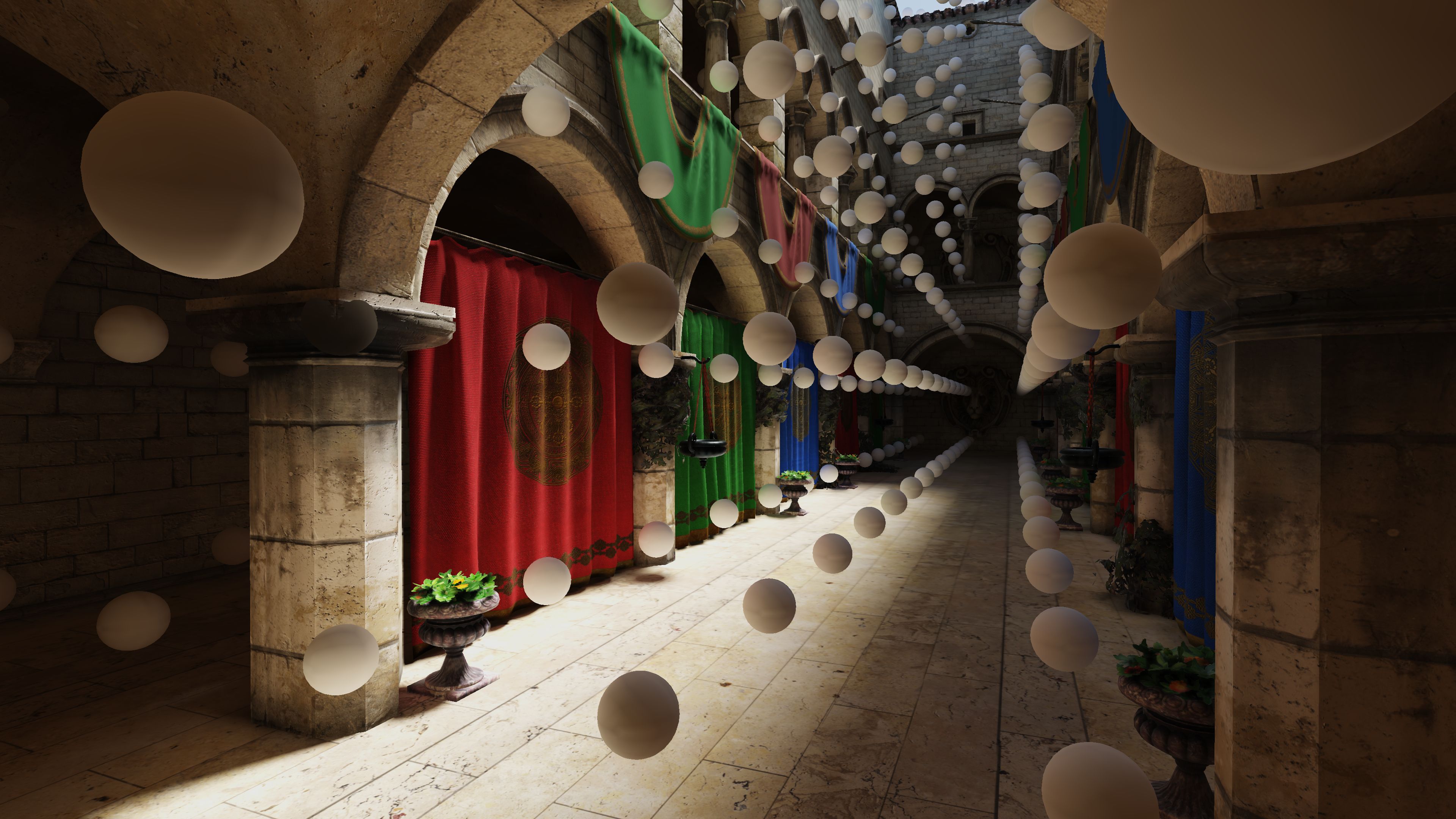
Global Illumination
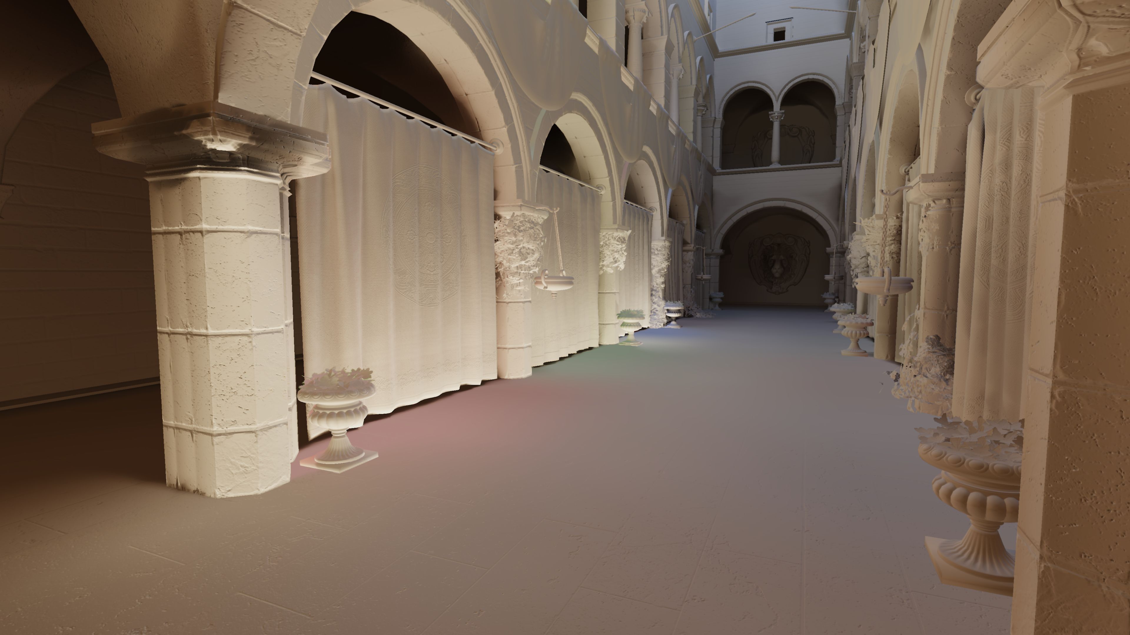
Ray Traced Global Illumination
The GI implementation for this sample started off as a simple 1spp, 2-bounce path trace thing denoised using SVGF, but I was never satisfied with how noisy it was in disoccluded regions. And the performance was rather horrendous as well. So I decided to scrap that and look into Dynamic Diffuse Global Illumination [9].
The idea is quite simple: It’s basically a grid of irradiance probes that are updated in real-time using ray tracing with additional depth information stored at each probe to prevent light leakage. In my opinion, the true beauty of this technique is the fact that it requires zero denoising and looks very stable compared to the other techniques in this sample. But this stability comes at the cost of temporal lag, meaning that the GI takes time to adapt to fast moving light sources or geometry since we’re blending the probes with new information over time.
My implementation sticks quite close to the original so I’ll only be going over the optimizations I’ve made. If you’re unfamiliar with the technique, please read the paper and come back to this.
Probe Update
The accompanying code with the paper samples each ray direction and radiance result for each texel of a probe which as you can imagine takes a rather heavy toll on texturing, but this is unavoidable seeing as the sample does the probe update in a pixel shader.
// For each ray
for (int r = 0; r < num_rays; ++r)
{
    vec3  ray_direction      = texture(sRayDirections, coord).xyz;

    vec3  ray_hit_radiance   = texture(sRayRadiance, coord).xyz * energy_conservation;

    vec3 texel_direction = oct_decode(normalized_oct_coord(current_coord, PROBE_SIDE_LENGTH));

    float weight = max(0.0, dot(texel_direction, ray_direction));

    if (weight >= FLT_EPS)
    {
        result += vec3(ray_hit_radiance * weight);

        total_weight += weight;
    }
}
Since I’m using a compute shader it gave me plenty of room to optimize this. Since all the ray directions and radiance values need to be read by every texel in the probe, this seemed like the ideal place to make use of some shared memory. I made sure that each workgroup maps to a single probe and then created a small cache in shared memory for the ray direction and radiance/depth values and populate this cache in parallel with each thread loading in a single value. My local workgroup size for this was 8x8x1 for radiance probes and 16x16x1 for depth probes.
Having 64 rays per frame per probe maps perfectly in the case of radiance probes since each workgroup has 8x8=64 threads, but if the ray count is higher surely we can make the cache larger and make some threads load more than one value right? Sure, while that is possible it is not a good idea because using too much shared memory will just reduce GPU occupancy resulting in worse performance. The solution I came up with that suits any number of rays is to keep the cache size constant and gather the rays in multiple batches as seen below.
vec3  result       = vec3(0.0f);
float total_weight = 0.0f;

uint remaining_rays = ddgi.rays_per_probe;
uint offset = 0;

while (remaining_rays > 0)
{
    uint num_rays = min(CACHE_SIZE, remaining_rays);

    populate_cache(relative_probe_id, offset, num_rays);

    barrier();

    gather_rays(current_coord, num_rays, result, total_weight);

    barrier();

    remaining_rays -= num_rays;
    offset += num_rays;
}

if (total_weight > FLT_EPS)
    result /= total_weight;
Border Update
The border update step which is required in order to prevent ugly artefacts when sampling the edges of the probes using bilinear filtering is often not well described so I’ll go into detail on how I tackled it in this sample. I started off by looking the diagrams from [10] which shows which probe texels need to be copied for which border texel and went ahead and generated the offsets for these coordinates relative to the beginning coordinate of the probe within the probe texture. Using this makes the copy super straightforwad with a couple of lines.
void copy_texel(ivec2 current_coord, uint index)
{
    ivec2 src_coord = current_coord + g_offsets[index].xy;
    ivec2 dst_coord = current_coord + g_offsets[index].zw;

#if defined(DEPTH_PROBE)
    imageStore(i_OutputDepth, dst_coord, imageLoad(i_OutputDepth, src_coord));
#else
    imageStore(i_OutputIrradiance, dst_coord, imageLoad(i_OutputIrradiance, src_coord));
#endif
}
The entire thing is done within a single compute shader with a local workgroup size equalling 4x the probe side length. This allows every border texel on the sides to be copied by its' own thread. However the 4 corner texels get missed out because of this, so I just repurposed the first 4 threads to copy those over.
const ivec2 current_coord = (ivec2(gl_WorkGroupID.xy) * ivec2(PROBE_SIZE_WITH_BORDER)) + ivec2(1);

copy_texel(current_coord, gl_LocalInvocationIndex);

// Copy corner texels
if (gl_LocalInvocationIndex < 4)
    copy_texel(current_coord, (NUM_THREADS_X * NUM_THREADS_Y) + gl_LocalInvocationIndex);
Probe Sampling
Since sampling the probe grid needs 16 samples per pixel (8 irradiance, 8 depth), it’s pretty expensive when doing it in the deferred shading pass at full resolution. Since Diffuse GI is rather low-frequency, we can get away with sampling it at a much much lower resolution. In my sample, I’m sampling the probe grid in a separate pass at half resolution and doing a bilateral upsample to bring it back up to full resolution while preserving edges. This seemd to work rather nicely and runs much much faster than the full resolution equivalent with nearly identical visual quality.
Performance
- NVIDIA GeForce RTX 2070 SUPER
- 1920x1080 Window Resolution
- 3960 Probes
- 256 Rays Per Probe
- Sponza Scene
| Pass | Original | Optimized |
|---|---|---|
| Ray Trace | 3.47 ms | 3.34 ms |
| Irradiance Update | 0.46 ms | 0.28 ms |
| Depth Update | 1.78 ms | 1.06 ms |
| Border Update | 0.05 ms | 0.05 ms |
| Sample Probe Grid | 0.88 ms | 0.88 ms |
| Total | 6.66 ms | 5.65 ms |
Conclusion
So these were some of the noteworthy things I’ve learned throughout the process of making this sample. Hope this post helped you understand what the code actually does and maybe even gave you a few ideas on how to tweak your own Hybrid Rendering Pipelines. There are plenty more techniques to try out such as Ray Traced Translucency, Transparent Shadows and Order Independent Transparency to name a few. Also a simplified denoiser that doesn’t just use SVGF for everything would be nice! I might just save some of these for a future blog post. But until then, have fun with this sample!
References
- [1] Spatiotemporal Variance-Guided Filtering
- [2] Fast Denoising with Self Stabilizing Recurrent Blurs
- [3] A Low-Discrepancy Sampler that Distributes Monte Carlo Errors as a Blue Noise in Screen Space
- [4] Using Blue Noise For Raytraced Soft Shadows
- [5] AMD FidelityFX Shadow Denoiser
- [6] Reprojecting Reflections
- [7] Accurate Real-Time Specular Reflections with Radiance Caching
- [8] Hybrid Rendering for Real-Time Ray Tracing
- [9] Dynamic Diffuse Global Illumination with Ray-Traced Irradiance Fields
- [10] Engine Work: Global Illumination with Irradiance Probes